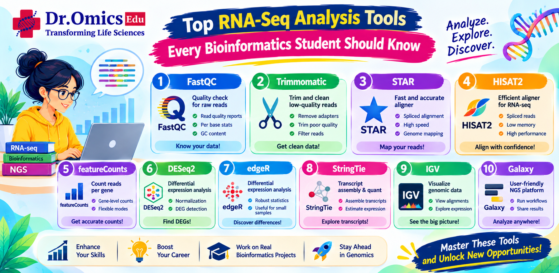
Top RNA-Seq Analysis Tools Every Bioinformatics Student Should Know
Priyanka Bhore · · Updated
Introduction
RNA sequencing (RNA-seq) is one of the most widely used techniques for studying gene expression and understanding biological processes. It helps researchers identify which genes are expressed, compare expression levels between experimental conditions, and investigate molecular changes associated with diseases.
However, RNA-seq generates millions of sequencing reads, making computational tools essential for processing and interpreting the data.
Different tools are used at different stages of the RNA-seq workflow, including quality control, read alignment, expression quantification, differential expression analysis, and functional interpretation.
For students learning bioinformatics, understanding these tools is an important step toward working with real-world transcriptomics datasets.
In this blog, we will explore the major RNA-seq tools, their applications, and how they work together in a typical gene expression analysis pipeline.
1. FastQC – Quality Control of Raw Reads
FastQC is commonly used as the first step in RNA-seq analysis. It evaluates the quality of raw sequencing reads stored in FASTQ files.
It generates reports containing information about:
- Per-base sequence quality.
- GC content distribution.
- Adapter contamination.
- Sequence duplication.
- Read length distribution.
Example command:
fastqc sample_R1.fastq.gz sample_R2.fastq.gz -o fastqc_results/
FastQC helps researchers identify potential sequencing quality issues before starting downstream analysis. It does not modify the original FASTQ files.
2. Trimmomatic and fastp – Read Trimming
Sequencing reads may contain adapter sequences and low-quality bases that can affect downstream alignment.
Trimmomatic and fastp are commonly used to remove unwanted sequences and filter low-quality reads.
Example using fastp:
fastp \
-i sample_R1.fastq.gz \
-I sample_R2.fastq.gz \
-o trimmed_R1.fastq.gz \
-O trimmed_R2.fastq.gz \
-h fastp_report.html
fastp performs adapter trimming, quality filtering, and generates an HTML quality report.
Trimming parameters should be selected based on the sequencing quality and experimental requirements.
3. HISAT2 and STAR – RNA-Seq Read Alignment
After quality control, sequencing reads are mapped to a reference genome.
Unlike DNA sequencing, RNA-seq alignment must account for introns because mature RNA transcripts are formed after intron removal through splicing.
Two commonly used tools are HISAT2 and STAR.
HISAT2
HISAT2 is a fast and memory-efficient splice-aware aligner used for mapping RNA-seq reads to a reference genome.
Example command:
hisat2 -x genome_index \
-1 sample_R1.fastq.gz \
-2 sample_R2.fastq.gz \
-S sample.sam
Here, -x specifies the reference genome index, while -1 and -2 represent paired-end reads.
STAR
STAR (Spliced Transcripts Alignment to a Reference) is another widely used RNA-seq aligner. It is known for its fast and accurate mapping of splice junctions.
Example command:
STAR \
--genomeDir genome_index \
--readFilesIn sample_R1.fastq.gz sample_R2.fastq.gz \
--outFileNamePrefix sample_
For compressed FASTQ files, STAR can also use --readFilesCommand zcat.
HISAT2 vs STAR
Both tools are suitable for splice-aware RNA-seq alignment.
- HISAT2 is generally memory-efficient and uses a hierarchical indexing strategy.
- STAR is known for high-speed alignment and detailed splice-junction detection, but can require substantial memory during genome indexing.
The choice depends on available computational resources, dataset size, and analysis requirements.
4. featureCounts – Gene Expression Quantification
Once reads are aligned, researchers need to determine how many reads map to each gene.
featureCounts, part of the Subread package, is commonly used for gene-level read quantification.
It uses alignment files and a gene annotation file, such as GTF, to count reads assigned to genomic features.
Example command:
featureCounts \
-a annotation.gtf \
-o gene_counts.txt \
sample.bam
The output contains read counts for genes and can be used for downstream differential expression analysis.
Accurate quantification depends on the reference genome, annotation file, strandedness, and appropriate handling of paired-end reads.
5. DESeq2 – Differential Gene Expression Analysis
DESeq2 is an R package widely used to identify differentially expressed genes between experimental conditions.
It works with raw gene-level count data and uses statistical modelling to estimate changes in gene expression.
For example, researchers may compare gene expression between healthy and diseased samples to identify genes associated with a particular condition.
DESeq2 tutorial: Basic workflow
Step 1: Load the package
library(DESeq2)
Step 2: Create a DESeqDataSet
dds <- DESeqDataSetFromMatrix(
countData = count_matrix,
colData = sample_metadata,
design = ~ condition
)
Here:
- count_matrix contains raw gene counts.
- sample_metadata contains sample information.
- design = ~ condition specifies the experimental variable being studied.
Step 3: Perform differential expression analysis
dds <- DESeq(dds)
Step 4: Extract results
res <- results(dds)
head(res)
The results include:
- log2FoldChange: Magnitude and direction of expression change.
- pvalue: Statistical significance.
- padj: Adjusted p-value accounting for multiple testing.
Genes with suitable adjusted p-values and biologically meaningful fold changes can be selected for further investigation.
6. edgeR – Differential Expression Analysis
edgeR is another popular R package used for differential expression analysis of RNA-seq count data.
It uses statistical methods based on the negative binomial distribution to model biological variability in sequencing data.
A basic edgeR workflow includes:
- Creating a DGEList object.
- Filtering lowly expressed genes.
- Normalizing count data.
- Estimating dispersion.
- Performing statistical testing.
- Identifying differentially expressed genes.
Example code:
library(edgeR)
y <- DGEList(counts = count_matrix)
keep <- filterByExpr(y, group = group)
y <- y[keep, , keep.lib.sizes = FALSE]
y <- calcNormFactors(y)
design <- model.matrix(~ group)
y <- estimateDisp(y, design)
fit <- glmQLFit(y, design)
test <- glmQLFTest(fit, coef = 2)
topTags(test)
edgeR is particularly useful for experiments with biological replicates and complex experimental designs.
DESeq2 vs edgeR
Both tools are widely accepted for RNA-seq differential expression analysis.
- DESeq2: Uses a negative binomial model with its own normalization and dispersion estimation framework.
- edgeR: Provides flexible statistical modelling and robust methods for handling different experimental designs.
Neither tool is universally better. The choice depends on the study design, analysis requirements, and the researcher's preferred workflow.
7. Additional Tools Every RNA-Seq Student Should Know
Apart from the major tools discussed above, several other tools are useful in transcriptomics research.
Salmon: Performs transcript-level abundance estimation using lightweight mapping approaches.
StringTie: Used for transcript assembly and abundance estimation from RNA-seq alignment data.
MultiQC: Combines quality-control reports from multiple bioinformatics tools into a single report.
IGV (Integrative Genomics Viewer): Allows researchers to visually inspect sequencing alignments and gene expression evidence across genomic regions.
clusterProfiler: An R package used for functional enrichment analysis, including Gene Ontology and pathway analysis.
These tools help extend RNA-seq analysis beyond basic alignment and differential expression.
8. A Typical RNA-Seq Analysis Workflow
A basic bulk RNA-seq workflow connects these tools in the following order:
- Raw FASTQ files: Obtain sequencing reads.
- Quality control: Use FastQC and MultiQC.
- Read trimming: Use fastp or Trimmomatic when required.
- Alignment: Map reads using HISAT2 or STAR.
- Quantification: Use featureCounts for gene-level counts or Salmon for transcript-level abundance estimation.
- Differential expression: Use DESeq2 or edgeR with appropriate count data.
- Functional enrichment: Use clusterProfiler to investigate biological pathways and Gene Ontology terms.
- Visualization: Generate heatmaps, volcano plots, PCA plots, and expression profiles.
The workflow may differ depending on whether the analysis uses genome alignment or transcript-level quantification. For example, Salmon-based workflows can be used without conventional genome alignment.
Conclusion
RNA-seq analysis involves several computational steps, and each requires specialized bioinformatics tools. FastQC and fastp support quality assessment and preprocessing, HISAT2 and STAR perform splice-aware alignment, and featureCounts and Salmon help quantify gene or transcript expression.
For differential expression analysis, DESeq2 and edgeR are among the most widely used tools in transcriptomics research.
For bioinformatics students, learning these tools through practical datasets is more valuable than simply memorizing commands. Understanding how each tool works and how its output connects to the next analysis step provides a strong foundation for working with real-world RNA-seq projects.
