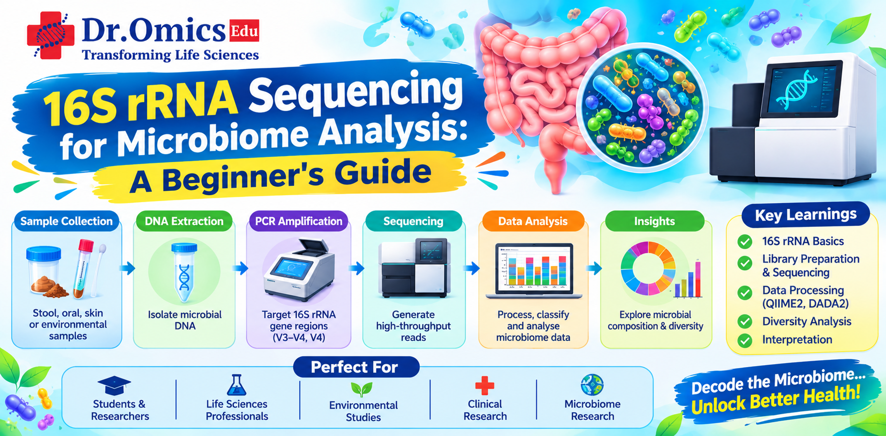
16S rRNA Sequencing for Microbiome Analysis: A Beginner's Guide

Introduction

Microorganisms such as bacteria and archaea play an important role in human health, agriculture, environmental balance, and several biological processes. These microbial communities are collectively known as the microbiome. Understanding their composition and diversity helps researchers investigate conditions such as gut disorders, infections, soil health, and environmental changes.

However, studying microorganisms individually using traditional culture-based methods can be challenging because many microbes cannot be easily grown under laboratory conditions. This is where sequencing-based approaches become useful.

16S rRNA gene sequencing is one of the most widely used techniques for studying bacterial and archaeal communities. It allows researchers to identify microorganisms in a sample by sequencing selected regions of the 16S ribosomal RNA gene.

In this beginner's guide, we will understand the principle of 16S rRNA sequencing, explore its applications, and learn how a typical microbiome analysis workflow is performed using bioinformatics tools such as QIIME 2.

1. What Is 16S rRNA Gene Sequencing?

The 16S rRNA gene is present in bacteria and archaea and encodes the RNA component of the small ribosomal subunit.

It is commonly used for microbial identification because it contains two important types of regions:

• Conserved regions: Similar across many bacterial groups, making them useful for designing universal primers.
• Variable regions: Differ between microorganisms and help distinguish bacterial taxa.

The gene contains nine variable regions, known as V1 to V9. Researchers select specific variable regions, such as V3–V4 or V4, for amplification and sequencing.

For example, if a researcher wants to study the bacterial composition of human gut samples, the 16S rRNA gene can be amplified from extracted microbial DNA. The resulting amplicons are sequenced, and the reads are analyzed to identify the microorganisms present.

Unlike shotgun metagenomic sequencing, which sequences DNA from across the microbial community, 16S sequencing focuses on a specific marker gene.

2. How Does 16S rRNA Sequencing Work?

The overall process involves laboratory preparation followed by computational analysis.

A typical workflow includes the following steps:

Step 1: Sample collection

Samples may be collected from different sources, including:

• Human stool samples
• Soil samples
• Water samples
• Food samples
• Environmental surfaces

For gut microbiome studies, stool samples are commonly used to investigate bacterial community composition.

Step 2: DNA extraction

Total microbial DNA is extracted from the collected sample. The quality and quantity of DNA are checked before proceeding.

Step 3: PCR amplification

Selected variable regions of the 16S rRNA gene are amplified using specific primers.

For example, V3–V4 primers are frequently used in bacterial community studies.

Step 4: Library preparation and sequencing

Sequencing adapters and sample-specific barcodes are added to the amplified DNA. The prepared libraries are then sequenced, commonly using Illumina sequencing platforms.

Step 5: Bioinformatics analysis

The generated sequencing reads are processed to remove low-quality sequences, identify microbial taxa, and calculate microbial diversity.

This final stage is known as microbiome bioinformatics analysis.

3. Understanding the 16S rRNA Bioinformatics Workflow

After sequencing, the output generally consists of FASTQ files containing DNA sequences and their quality scores.

These files are used for downstream analysis.

A typical microbiome analysis workflow includes:

1. Importing raw sequencing reads.
2. Checking sequence quality.
3. Removing low-quality reads and sequencing errors.
4. Identifying Amplicon Sequence Variants (ASVs).
5. Assigning taxonomy to identified sequences.
6. Calculating alpha and beta diversity.
7. Performing statistical comparisons between groups.
8. Visualizing microbial community composition.

Several tools are available for these steps, but QIIME 2 is one of the most widely used platforms for 16S rRNA analysis.

4. QIIME 2 Tutorial: Basic Steps for 16S rRNA Analysis

QIIME 2 is an open-source bioinformatics platform designed for microbiome research. It provides tools for processing sequencing data, performing diversity analysis, assigning taxonomy, and generating visualizations.

It is particularly useful for beginners because it provides a structured workflow for microbiome analysis.

Step 1: Import sequencing data

QIIME 2 supports different input formats. Before importing FASTQ files, researchers need to organize the reads according to the selected import format.

For example, paired-end reads may be supplied as forward and reverse FASTQ files.

A typical import command for paired-end demultiplexed reads is:

qiime tools import \

  --type 'SampleData[PairedEndSequencesWithQuality]' \

  --input-path manifest.csv \

  --output-path demux-paired-end.qza \

  --input-format PairedEndFastqManifestPhred33V2

Here:

• manifest.csv contains sample IDs and FASTQ file paths.
• --type specifies the type of sequencing data.
• --output-path defines the QIIME 2 artifact to be generated.

QIIME 2 uses .qza files to store analysis data and .qzv files for visualizations.

Step 2: Check sequencing quality

Before processing the reads, researchers should examine their quality profiles.

qiime demux summarize \

  --i-data demux-paired-end.qza \

  --o-visualization demux-summary.qzv

This generates a visualization containing read counts and per-base quality information.

Based on the quality profiles, researchers can decide where to trim low-quality regions.

Step 3: Denoising using DADA2

DADA2 is commonly used in QIIME 2 to remove sequencing errors and identify Amplicon Sequence Variants (ASVs).

ASVs represent unique biological sequences inferred after correcting for sequencing errors.

qiime dada2 denoise-paired \

  --i-demultiplexed-seqs demux-paired-end.qza \

  --p-trim-left-f 0 \

  --p-trim-left-r 0 \

  --p-trunc-len-f 240 \

  --p-trunc-len-r 200 \

  --o-table feature-table.qza \

  --o-representative-sequences rep-seqs.qza \

  --o-denoising-stats denoising-stats.qza

The trimming and truncation values shown are examples. Actual values should be selected after examining the quality plots and ensuring that sufficient overlap remains for paired-end read merging.

This step generates:

• Feature table: Records the abundance of each ASV across samples.
• Representative sequences: Contains the DNA sequence corresponding to each ASV.
• Denoising statistics: Summarizes how many reads passed through each processing stage.

Step 4: Assign taxonomy

After identifying ASVs, the next step is to determine which microorganisms they represent.

QIIME 2 supports taxonomic classification using reference databases such as SILVA.

qiime feature-classifier classify-sklearn \

  --i-classifier silva-classifier.qza \

  --i-reads rep-seqs.qza \

  --o-classification taxonomy.qza

The classifier must be trained using a compatible reference database and the appropriate primer or amplicon region.

Taxonomic classification can identify microorganisms at different levels, including phylum, class, order, family, genus, and sometimes species.

However, 16S sequencing does not always provide reliable species-level identification.

Step 5: Perform diversity analysis

Microbial diversity is an important part of microbiome research. It helps researchers understand how microbial communities differ within and between samples.

Two major types of diversity analysis are commonly performed.

Alpha diversity

Alpha diversity measures microbial diversity within an individual sample.

Common metrics include:

• Observed features: Number of unique ASVs detected.
• Shannon index: Considers both richness and evenness.
• Simpson index: Measures diversity while accounting for dominance.

Beta diversity

Beta diversity measures differences in microbial community composition between samples.

Common distance metrics include:

• Bray–Curtis dissimilarity
• Jaccard distance
• Unweighted UniFrac
• Weighted UniFrac

For example, researchers may compare gut microbiome samples collected from healthy individuals and patients to investigate differences in microbial community composition.

QIIME 2 provides visualization tools such as principal coordinate analysis (PCoA) to explore beta diversity patterns.

5. Understanding Microbiome Analysis Results

Once the analysis is complete, researchers need to interpret the results biologically.

Some commonly generated outputs include:

Taxonomic composition plots: These plots show the relative abundance of microbial groups at different taxonomic levels.

Alpha diversity plots: These help compare within-sample diversity between experimental groups.

PCoA plots: These provide a visual representation of differences in microbial communities across samples.

Differential abundance analysis: This identifies microbial features whose abundance differs between groups. Statistical methods should account for the characteristics of microbiome data, including compositionality and multiple testing.

For example, a study comparing healthy and diseased individuals may identify differences in the relative abundance of certain bacterial groups. Such findings can help generate hypotheses about possible relationships between microbial communities and disease.

Importantly, differences in relative abundance do not automatically demonstrate that a microorganism causes a disease or provides a health benefit.

6. 16S rRNA Sequencing vs Shotgun Metagenomics

Both 16S sequencing and shotgun metagenomics are used to study microbial communities, but they differ in their sequencing approach and the information they provide.

16S rRNA sequencing targets a specific bacterial or archaeal marker gene, whereas shotgun metagenomics sequences DNA from across the microbial community.

The main differences are:

• Target: 16S focuses on the 16S marker gene; shotgun metagenomics analyzes broader microbial DNA.
• Microbial identification: 16S is mainly used for bacterial and archaeal taxonomic profiling, while shotgun sequencing can also support identification of fungi, viruses, and other organisms when suitable reference data and analysis methods are available.
• Functional analysis: 16S provides limited functional information, often through prediction methods. Shotgun metagenomics can directly identify genes and potential metabolic pathways.
• Cost and computational requirements: 16S is generally less expensive and requires fewer computational resources than deep shotgun metagenomic sequencing.

The choice depends on the research question, sample type, budget, and required level of biological information.

7. Applications of 16S rRNA Sequencing

16S rRNA sequencing is used in several areas of biological and biomedical research.

• Gut microbiome research: Studying bacterial communities associated with digestion, health, and disease.
• Environmental microbiology: Investigating microbial diversity in soil, freshwater, oceans, and other environments.
• Agriculture: Understanding soil microbial communities and their possible relationships with plant growth and crop health.
• Food microbiology: Monitoring bacterial communities involved in food production, fermentation, and spoilage.
• Clinical research: Investigating microbial community changes associated with different health conditions.

These applications make 16S rRNA sequencing an important technique in modern microbiome research.

Conclusion

16S rRNA gene sequencing provides a practical and widely used approach for understanding bacterial and archaeal community composition. From sample collection and DNA extraction to sequencing, denoising, taxonomic classification, and diversity analysis, every step contributes to generating meaningful microbiome insights.

Tools such as QIIME 2 and DADA2 make it possible to process sequencing reads and perform detailed microbial community analysis without developing an entire bioinformatics pipeline from scratch.

For beginners entering microbiome research, understanding the 16S workflow is an excellent starting point before exploring advanced shotgun metagenomics and functional microbiome analysis.

Learning these concepts through practical datasets and hands-on bioinformatics workflows can also provide a strong foundation for anyone interested in a metagenomics course or a career in microbiome bioinformatics.