Targeted metagenomics 101: 16S rRNA to shotgun sequencing step by step

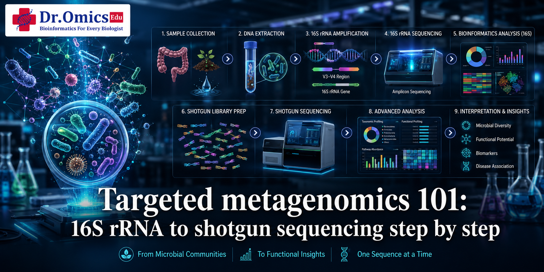
The microscopic world inside and around us plays a vital role in human health, agriculture, and ecology. To study these complex environments, scientists rely on metagenomics—the study of genetic material recovered directly from environmental samples.

If you are a student or a researcher entering this field, navigating a metagenomics workflow beginners pipeline can feel overwhelming. The first and most critical choice you will face is deciding whether to look at a specific genetic marker or to sequence everything in your sample.

Difference Between Targeted and Shotgun Metagenomics

Before diving into the computational steps, it is essential to understand the structural differences between the two main strategies used in microbial community analysis.

1. Targeted (Amplicon) Metagenomics

This approach targets a specific hypervariable marker gene present across all target organisms. For bacteria, the absolute standard is the 16S rRNA sequencing guide architecture. The 16S rRNA gene contains highly conserved regions (which allow universal primers to bind) interspersed with nine hypervariable regions ($V1 - V9$) that act as unique evolutionary fingerprints.

This method is highly cost-effective and works exceptionally well even with low-quality or host-contaminated samples. However, it only tells you who is there (taxonomic profiling), not what they are doing (functional profiling).

2. Shotgun Metagenomics

Instead of focusing on a single marker gene, shotgun sequencing breaks all the DNA in a sample into tiny fragments and sequences everything randomly. This gives you a complete view of the entire genomic ecosystem, allowing you to sequence bacteria, viruses, fungi, and micro-eukaryotes simultaneously.

Shotgun sequencing allows you to map metabolic pathways and functional genes, answering both who is there and what they are capable of doing. The trade-off is that it requires significantly more computational power, deeper sequencing, and higher budgets.

The Metagenomics Pipeline Step by Step for Beginners

To take raw data from a sequencing machine and turn it into beautiful microbial diversity plots, you will follow a highly structured 16S amplicon sequencing workflow. Here is how to analyze your data sequentially:

Step 1: Quality Control and Demultiplexing

Raw sequencing data contains adapters and low-quality bases. Using metagenomics data analysis tools 2026 standards, researchers use software like FastQC or Trimmomatic to clean up the reads. Demultiplexing ensures that reads are properly assigned back to their original samples based on their unique barcode sequences.

Step 2: Denoising and Grouping (The OTU vs. ASV Analysis Difference)

Once the reads are clean, they must be grouped to identify distinct microbial types. Historically, researchers grouped sequences that were 97% identical into Operational Taxonomic Units (OTUs).

Today, modern pipelines favor Amplicon Sequence Variants (ASVs). The OTU ASV analysis difference comes down to exact single-nucleotide resolution. ASVs treat every unique sequence string as its own entity and discard sequencing errors using advanced statistical models (like DADA2). This allows for much higher taxonomic precision and makes it easy to compare datasets across different labs.

Step 3: Taxonomic Classification with QIIME2

If you are learning how to analyze 16S rRNA sequencing data with QIIME2, this is where the magic happens. QIIME2 is the gold standard framework for an amplicon sequencing tutorial. You train a Naive Bayes classifier on a reference database (such as SILVA or GreenGenes) to automatically assign a kingdom, phylum, class, order, family, genus, and species tag to your ASVs.

Step 4: Diversity Analysis

Once your taxonomic profile is built, you evaluate the structure of your microbial community using two core ecological metrics: alpha beta diversity metagenomics.

• Alpha Diversity: Measures the variety and abundance of microbes within a single sample. Common metrics include Observed Features (richness) and the Shannon Index (evenness).
• Beta Diversity: Measures the structural differences between different samples or groups (e.g., comparing the gut microbiome of healthy individuals vs. patients). This is visualized using Principal Coordinate Analysis (PCoA) plots based on distances like UniFrac or Bray-Curtis.

Final Thoughts

Whether you begin your journey with a focused QIIME2 16S analysis or dive straight into assembly-driven shotgun workflows, mastering a targeted metagenomics tutorial layout is foundational for modern life science research. By combining taxonomic classifications with robust diversity metrics, you can transform massive sequence files into powerful biological conclusions that advance our understanding of microbial ecology.